UNIGIT RIGOROUS GRATING SOLVER
VERSION 2.02.02
USER MANUAL
Developed
by:
Osires
& Optimod
Schillerstrasse
19
D -
9693 Ilmenau
GERMANY
phone:
+49 03677 46562
cell
phone: +49 162 9067015
email:
support@unigit.com
Change Record
changes versus previous versions of Unigit Tab
|
Reason for Change/ Extension |
Section(s) |
Page(s) |
|
This
is the first version of Unigit Tab |
|
|
|
For
previous versions refer to Manual Unigit version 2.02.01 |
|
|
|
|
|
|
Table of Content
changes
versus previous versions of Unigit Tab
2.1. Introductory Remarks & Introduction Tab
3.1. Layer Editor for 1D RCWA (1D)
3.1.2. Rayleigh-Fourier Polygon.
3.1.3. Rayleigh-Fourier Polygon.
3.1.4. RCWA Slice, hard transition
3.1.5. RCWA Slice, soft transition
3.2. Layer Editor for 1D C-Method (1C)
3.2.1. Thin film (plane interface)
3.3. Layer Editor for 2D RCWA (2D)
3.4. Layer Editor for 2D C-Method (2C)
5.2. Retrieving input information
5.3. Retrieving stack (grating) information
5.4. Retrieving computation results
6.2. Calculation of the Diffraction Angles
1.
Introduction
Unigit is a rigorous diffraction solver for 2D (1D periodic) or 3D (2D periodic) multilayer stacks (see Fig. 1). It runs on PC with Windows NT, Windows 2000, Windows XP, Vista and Windows 7 both 32 and 64 bit machines. The schema in Fig. 1 gives an idea what types of complex patterns can be solved with Unigit.
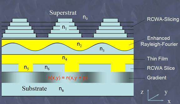
Fig. 1: Schematic representation of a multilayer stack
Unigit V2.XX.XX comprises three basic solution algorithms:
- the
Rigorous Coupled Wave Approach (RCWA) a.k.a. Modal Method with Fourier
Expansion (see e.g., /1/, /2/),
- the
Chandezon method (C-method) a.k.a. Coordinate Transformation Method (see
e.g., /8/ & /9/),
- and
the Rayleigh Fourier Method (/3/) which is not rigorous.
Presently, algorithms one and three are
embedded in the same S-matrix algorithm (see e.g., /4/) ensuring a high degree
of stability as well as flexibility while the C-method is implemented
separately. It is planned however to merge all three algorithms into one frame
for upcoming versions. The algorithms can be applied layer wise, i.e., one
layer can be treated with Rayleigh-Fourier and another layer with RCWA. The
implementation of RCWA was done in compliance with Lifeng Li’s factorization
rules (see e.g., /5/) to insure accurate results. The 2D algorithm follows
closely Lifeng Li’s paper /6/. In addition, it offers the choice of the Lalanne
method /7/ instead of the Li Method. The implementation of the C-method
followed mainly the description in /9/ as well as some sophisticated schemas to
couple the fields between non-parallel interfaces. The C-method is an ideal
supplement to the RCWA. Its preferred application cases are profiles with
shallow slopes made from high contrast materials. A particular case are Echelle
gratings. Some examples proving the superiority of the C-method in these cases
are discussed in /10/.
Unigit consists of a Graphical User Interface
(GUI) and five computation kernels. The computation kernels are:
- Unigit_1D.exe:
A solver for one-dimensional (1D) or line/ space gratings (with orthogonal
and/or slanted layers) in classical mount based on RCWA and
Rayleigh-Fourier method,
- Unigit_1C.exe:
A solver for one-dimensional, (non/parallel) multi-layer gratings in classical mount based on the C-method,
- Unigit_1DC.exe:
A solver for one-dimensional (1D) or line/ space gratings (with orthogonal
and/or slanted layers) in conical mount based on RCWA,
- Unigit_1CC.exe:
A solver for one-dimensional, (non/parallel) multi-layer gratings in conical mount based on the C-method,
- Unigit_2D.exe:
A solver for non-orthogonal crossed (2D) gratings based on RCWA,
- Unigit_2DSX.exe:
A solver for non-orthogonal crossed (2D) gratings with symmetry
acceleration for oblique incidence (symmetry conditions must be met) –
speed up factor up to 4x (8x for one polarisation).
- Unigit_2DS0.exe:
A solver for non-orthogonal crossed (2D) gratings with symmetry
acceleration at normal incidence (symmetry conditions must be met) – speed
up factor up to 32x (64x for one polarisation),
- Unigit_2C.exe: A solver for
multilayer (parallel), crossed gratings based on the C-method.
The eight computation kernels can be utilized
without the Unigit-GUI by embedding it in user applications. This can be done
for example with Matlab, Python, Visual Basic,
C++ or C#.
In order to speed up the computation, Unigit
enables the parallel threading of loops. This feature is particularly
recommended to run slow 2D computations on multi-core machines. For instance, a
speed up factor of about 4-6 will become possible for a dual quad-core machine.
The parallel threading can be activated in the Settings tab (for more details
see section 2). Moreover, the simulation of
symmetric crossed gratings illuminated in a symmetric setup may be accelerated
by taking advantage of these symmetries (see section 2.2).
2.
Tab Based Control Board
2.1.
Introductory
Remarks & Introduction Tab
The new (tab page based) control board is
activated immediately after the UNIGIT program is started. It appears as shown in
Fig. 1.
Fig. 1: New Central Control Board of Unigit
Mainly, the
tab control board serves for:
- The preparation of the input files of the
underlying Grating Solver Code,
- the launch of the Grating Solver and
- the graphical presentation of the
calculation results.
It consists
of seven tab pages:
- About Tab: Introduction, Starting Tab;
- Settings Tab: Offering basic settings that
apply to the whole program;
- Excitation Tab: Defining the excitation
conditions for the grating such as wavelength, AOI, truncation, type of
mount etc. and provides choices for loops over these parameters;
- Grating Stack Tab: Selection or Assembling
of multi-layer stack gratings (RCWA or C-method, 1D or 2D) – replaces the
Stack Editor of former versions;
- Output Control Tab: Defining how to output
the results – replaces the output editor of former versions;
- Run Tab: Starting the computation (enables
additional setting for 2D computation such as choice of symmetry
acceleration);
- Show Results Tab: Drawing results as
diagram, Open result file with Notepad, Passing result to Excel.
These tabs
and their order are designed to reflect the work flow of the code for
preforming grating computations.
Besides, the basic operation modes of UNIGIT
can be selected just by selecting either a regular stack file (extensions
“.ust” preferred though you can use other, e.g. “.txt” have been used with
older versions of UNIGIT) or a UNIGIT project file (extension “.upr”).
Accordingly, there are two basic modes how Unigit can be operated:
- The regular mode,
- The project retrieval mode.
The following
sections are devoted to the regular mode. The project retrieval mode is
described in more detail in section 8.
Next, the
seven Tabs are discussed in more detail.
The
Introduction Tab is already shown in Fig. 1. At the left side, it shows some
information about the release and built number of the Unigit code. To the
right, a link to the Unigit web page is provided followed by an email link to
our support. Moreover, a link to the Unigit manual is given as well a link to a
video presentation of the new release. Finally, the detected protection system
is shown to the right.
2.2.
Settings
Tab
The
settings tab (see ) provides some basic settings for the program that are
organised in five groups.
Fig. 2: Settings
Tab
These
groups shall be presented in more detail in the following.
2.2.1. Group Parallel Loop
This group (see
Fig. 3) contain the permission and the
settings to run parallel loops, i.e., the loop that is defined in the
Excitation Tab.
After activiation of the parallel looping mode,
two edit fields become active – the number (parallel) threads and the delay
time between the various thread launches. An arbitrary integer number greater
zero should be entered for the number of threads. The default is the number of
available computation cores. However, the entered value can be different. It is
recommended to find an optimum number (to achieve maximum computation speed) by
means of numerical experiments. The default value for the delay time is 50 ms.
It is recommended to increase this value if synchronization issues occur, i.e.,
single process threads fail.
Fig. 3: Parallel
Loop Group (Settings Tab)
2.2.2. Group Color Code
The color
tab settings are closely linked to the color coding of materials and n&k
files and will effect the cross section drawing in the Grating Stack Tab. The group
box (see Fig. 4) enables the loading and editing of
a color table. The color table itself is a simple Ascii-file that contains a
list with pairs of color-ID's (names) and assigned RGB color reference values.
The table can either be edited by Notepad (or another Ascii editor) or by means
of the built in color table editor.
Fig. 4: Color
Code Table (Settings Tab)
The color
table editor enables the viewing, changing and adding of color assignments to
n&k materials. In order to add an entrance, fill the material ID edit with
a new name of your choice and select a color by clicking the button next to Color.
Finally, append the new pair by clicking the ADD button or discard your choice by doing anything
else. After adding a new pair the total score will be increased by 1.
Currently, the elimination of an entrance is only possible via the Notepad
editor. Alternatively,
the color table can also be created and edited in a Notepad editor. An example
of a color table file is shown in Fig. 5.

Fig. 5: Example
of a color table file
2.2.3. Run Group
The run
group (see Fig. 6) comprises a few settings that
become active during and shortly after computation runs (performed from the Run
Tab).

Fig. 6: Run
Group (Settings Tab)
Currently,
there are 3 check boxes available in this group:
- Silent: if checked, the CMD window does
not appear during computation (often makes sense for large loops or
parallel loops), it has no effect if “no output file” is selected in the
Output Control Tab;
- Show Immediately: if checked, the selected
output file (see Output Control Tab) is opened directly after the
computation run and the results are displayed.
- Diagnosis: if checked, some additional
messages are shown that help to track down misfunctioning.
2.2.4. Stack File Group
The stack
file group (see ) contains some settings that become active in the Grating
Stack Tab.

Fig. 7: Stack
File Group (Settings Tab)
There are
three checkboxes:
- Use New File after Edit: currently
inactive;
- Parse when selected: if checked, the stack
file is parsed after selection (i.e., before loading in the stack editor
(part of the Grating Stack Tab) and inconsistencies are detected ad
reported;
- Safe after Notepad: if checked, the stack
file is updated after it has been opened with Notepad, if not checked, the
stack file is not automatically saved and the computation will run with
the state before opening (this is indicated by red color of the file path
display in the Grating Stack Tab).
2.2.5. Python Group
The Python
group box in the Settings Tab is provided for loading and editing a Python
script file to run Unigit.
2.3.
Excitation
Tab
The
Excitation Tab (see Fig. 8) is devised for defining the
excitation conditions for the grating computation. It offers means to run loops
over the excitation parameters.
Fig. 8: Excitation Tab
2.3.1. Loop Group
Especially,
the following parameters may be defined:
- The wavelength (to be entered in microns),
- the truncation number (i.e., the minimum
and maximum Rayleigh order to be kept in the diffraction matrix
algorithm),
- the (polar) incidence angle and
- the azimuthal incidence angle (This option
is activated only in the conical and 2D case).
A loop
option is linked to each of these four parameters. This means that the
computation will be performed for several values of this parameter defined by a
start, stop and step value.
Optionally,
one geometry parameter of the stack may be also integrated in the loop
selection. In order to do this, the particular parameter has to be indicated by
means of a dollar sign at the end of its line in the stack file. You can do
this by opening the file with the notepad button. The example in Fig. 9 shows the selection of the grating
thickness as a parameter.
![]()
Fig. 9: Activation
of a wild card loop (via $ sign)
The mark is
recognized automatically and an additional radio button together with input
field(s) pops up after saving the change and leaving the notepad editor. This
is shown in ???. If the “/d” box is checked, than the loop parameters are
related to the pitch, i.e., entering 0.2 at pitch 0.5 microns means 0.1 micron.
Fig. 10: Activated
and selected wild card loop
2.3.2.
Flexi
Loop
The looping
group permits already quite some versatility in terms of looping. However, it
is limited to the variation of just one parameter and to equidistant steps.
This can be overcome by the Flexi loop. In order to activate it, the Flexi loop
box has to be checked (see Fig. 11) and a loop control file (extension
.ulf) has to be loaded.
Fig. 11: Activated
Flexi Loop (Excitation Tab)
An example of an .ulf file is shown in Fig. 12. The parameters have to be listed
in exactly the order as shown in the figure. Furthermore, the total number of
parameter sets has to be entered in the second line (here 6). Beside of these
constraints, the parameter values in each line (corresponding to a parameter
set) are quite arbitrary within the range of physical values. Of course, single
loops can also be specified but as opposed to the single loop selection, a
variable step width can be invoked such as shown in the example of Fig. 12. Finally, the output parameter of
the set which shall be appear in the output file (parameter to be printed) can
also be selected via the radio buttons (theta_i in the example of Fig. 11).
Fig.
12: Example
of an Unigit Loop File (.ulf)
2.3.3.
Mount
Selection
The mount
selection offers two choices – the classical and conical mount. In the
classical mount, the incident beam remains in the grating plane (defined by the
grating vector which is perpendicular to the grating grooves and the normal vector
for 1D gratings). Whereas in the conical mount it can be outside. Different
solvers are required in 1D for the polarization modes do couple for conical
mount and don’t couple for classical mount. In this way, the selection
determines which solver has to be run (unigit_1D or unigit_1C for classical and
unigit_1DC or unigit_1CC for conical mount). It has to be noted, that
comparisons can be made for both solvers by selecting on the one hand classical
mount and on the other hand conical mount and setting Phi = 0°.
In general,
the mount doesn’t matter for 2D gratings. However, if unigit_2DSX shall be run
for symmetry acceleration, the corresponding check box “Sym Oblique” in the Run
Tab will be only available by choosing conical mount and setting Phi = 90° while
the unigit_2DS0 check box “Sym Normal” will only be available when choosing
classical mount and setting AOI = 0°.
2.4.
Grating
Stack Tab
The Grating
Stack Tab provides more or less the functionality of the former stack editor
(until version 2.02.01). In addition, a cross section drawing of the stack can
be shown optionally on the right hand side of the Tab as shown in Fig. 13. According to the dimensionality (1D or 2D) and to the solution
method (RCWA or C-method) there are 4 basic grating types available in Unigit.
The dimensionality and solution method can be chosen when creating a new
grating by clicking the wanted radio buttons. In case, a grating is selected
from a database, these options are detected from the grating file and set
automatically.
As long as
no valid grating is selected, it is indicated with red color in the stack file
group. Similarly, the color changes to red as soon as the grating is changed by
editing one of its parameters. In order to run the grating structure that is
exhibited in the grating editor on the left-hand side of the Tab, one has to
make sure to save it first. After successful saving, the color of the stack
file path turns into black.
In the
following subsections, first the basic features of the stack editor are
explained and then, the four basic grating types along with their implemented
layer types are presented.
Fig. 13: Grating
Stack Tab with cross section drawing of the multilayer stack
2.4.1.
Stack
Editor
The stack
editor is integrated into the Grating Stack Tab and facilitates the assembling
of arbitrary multilayer grating structures for each of the four basic grating
types. The types of layers to choose from are context sensitive, i.e., they
depend on the selected solver type and dimensionality. For the editing, a
number of buttons are arranged below the spreadsheet list.
There are
several feasibilities to assemble the stack.
- First, new layers can be inserted by
starting the layer editor clicking the INSERT
button.
- Second, an existing layer can be edited by
clicking the EDIT-button. This action
also launches the layer editor with the selected layer. In order to select
a layer, the cursor has to be positioned at the beginning of the associate
description line.
- Third, the order can be changed by moving
a marked layer up or down.
- Fourth, a layer can be deleted by marking
it and press the DELETE button.
- Layers can be marked by clicking with the
left mouse button and concurrently holding the CTRL or SHIFT key and saved
as a sequence file. The marked layers must not necessarily form a coherent
string, i.e., unmarked lines are permitted between marked lines.
- Marked layers can be copied or cut and
later pasted (this is also possible between different stacks for the
information is stored to the clipboard). For instance, HL (high low
index)-quarter wave stacks can be built in this way.
This
functionality can also be accessed via hot keys as follows:
- SELECT
STACK CTR-S,
- EDIT STACK - CTR-E,
- OUTPUT
EDITOR CTR-O,
- NEW STACK CTR-N,
- DIAGRAM
TOOL CTR-D,
- ADD FILE 2
Diagram CTR-A,
- SELECT
RESULT FILE CTR-R,
- SETTINGS
EDITOR CTR-P,
- CANCEL
UNIGIT CTR-BREAK,
- EXIT UNIGIT CTR-X,
- RUN - ALT-R.
2.4.2.
RCWA
1D stacks
For 1D
(line gratings) there are 5 basic types of layers:
- homogeneous flat layer (type 1),
- sinusoidal Rayleigh-Fourier layer (type
2),
- polygonal Rayleigh Fourier layer (type 3),
- discrete RCWA layer (type 4) and
- continuous RCWA (i.e., gradient) layer
(type 5).
In addition
to these basic layer types, so-called composite layers can be input:
- polygonal RCWA layer (type 6),
- sinusoidal RCWA layer (type 7),
- sliced multilayer (RCWA),
- sequence of layers (comprising an
arbitrary number of layers from type 1 through type 7 in an arbitrary
order).
A symbolic
layer stack comprising all these layer types is shown in Fig. 14.
As opposed to the sinusoidal or polygonal
Rayleigh-Fourier (/3/) layer, the corresponding composite layers are
automatically decomposed (that means sliced) into discrete RCWA slices of type
4 immediately before being processed. A sequence of layers (also called
sub-stack) has to be stored as a file in the same way as the total stack
description is stored. The only difference between a complete stack and a
sub-stack consists in the fact that the complete stack comprises beside the
stack data the grating period as well as the superstrate and substrate
description. Moreover, a hierarchy of sequences is not permitted, i.e., a
sub-stack must not contain another sub-stack. As for layer editing see section
layer editor.
Fig. 14: Example
for a RCWA 1D layer stack
2.4.3.
C-Method
1D Stack
This editor enables the assembling of stack
files for the C-method. An unlimited number of non-parallel interfaces is
permitted. The stack editor considers the
interface as a “layer” just like in the same way as it does for
Rayleigh-Fourier interfaces. This arises from the layer-wise processing of
RCWA-slices. Basically, the stack editor enables several choices:
- Plane interface;
- CCM polygon = polygonal
C-method interface;
- CCM sinus = sinusoidal C-method
interface;
- Parallel to previous: meaning
the interface is parallel to the one below;
- Sequential: not yet
implemented;
- CCM Trapezoid: special case of
CCM polygon (with 6 profile sampling points);
- CCM measurement: special case
of CCM polygon where the profile sampling points are obtained from a
measurement file;
- CCM Triangle: special case of
CCM polygon (with 3 profile sampling points);
The interface types are uniquely identified by
its names. Beside the corrugation of the layers, the distances and if existent
the material ID's are shown. Note, that there is no distance entrance for the
uppermost interface (because it would have no meaning). An example of a
multi-layer stack containing all different layer types is shown in Fig. 15.
Fig.
15: Example
for a C-method 1D grating stack
2.4.4.
RCWA
2D Stack
There are basically 6 types of layers:
- Thin Film,
- Patches (rectangular),
- Ellipse,
- 3D Cone,
- Fill 2D,
- Sequence.
Here, the
types: thin film, patch, ellipse and fill2d are genuine 2D layers whereas 3D
cone and sequence are composite 3D-shapes formed by the basic 2D types (i.e.,
all 4 types are possible for sequence and ellipse type is used for 3D cone).
An example
of a multi-layer stack containing all different layer types for a RCWA 2d stack
is shown in Fig. 16.
Fig. 16: Example
for a RCWA-method 2D grating stack
2.4.5. C-Method 2D Stack
There
are basically 4 types of interfaces for
c-method 2D:
- Parallel to Previous
- Pyramide
- Micro-Lens
- Fill 2C.
In the
current implementation, only one out of the types pyramide, micro-lens and
fill2c can be chosen as bottom interface. In addition, only one interface of
type “parallel to previous” can be put on top of it resulting in a maximum
number of two interfaces. Examples are provided in Fig. 17, Fig. 18 and Fig. 19.
Fig. 17: Example
of a 2C stack with a pyramid interface
Fig. 18: Example
of a 2C stack with a micro lens interface
Fig. 19: Example
of a 2C stack with an arbitrary interface (fill2C) load from a file
2.5.
Output
Control Tab
The output
format (or control) tab replaces the output editor window of former versions
(up to 2.02.01). The appearance of this tab is shown below in Fig. 20.
Fig. 20: Output
Format Tab Page
It contains 5 groups and a number of file
selection inputs in the lower part.
These groups are discussed in the following.
2.5.1.
Output
Files Group
This group
is located in the upper left of the tab page. Here, the following choices can
be made:
- selection where to write the
output to (radio buttons top left)
- “No output file” means the
result appears in the DOS window
- “All in one” means the result,
i.e., all selected diffraction orders are written into one file. This
file can be specified in the Central Control Board in the text box “Save
result in”.
- “Single Files” means that each
diffraction order is saved in a separate file. The file location is
specified as before, however, the name is used as a template and is
completed by different attachments depending on the order, whether it is
reflection or transmission, the polarisation and the type of output
information. It also depends on which solver was specified (1D or 2D).
Basically, the following coding is
used:
Assume the basic name as specified in the text
box is “test”. Then, the file name is testOXOY.MPP where
- OX is the diffraction order
in x-direction,
- OY is the diffraction order
in y-direction (is obsolete for 1D case and is skipped there),
- M is the mode, i.e., R for
reflection or T for transmission,
- PP is the polarisation, first
P for input and second P for output. P can either be E for TE or M for
TM polarisation. To give an example, cross polarisation from TE to TM is
characterized by PP = EM whereas TE polarisation is assigned by PP = EE.
The second P is obsolete for 1D classic case (there is no cross
polarisation) and is thus skipped.
- As an example, test00m1.tmm
means transmission of TM in 0./ -1. order (x/y).
- Selection of the Mode
(checkboxes transmission/reflexion),
- Selection whether to append the
results to existing file(s) or create new one(s).
2.5.2. Output Format Group
The group
is the second from left in the upper half of the page. In this group, the
numerical format of the outputted results can be defined.
There are
the following choices:
- Select whether to output
efficiencies in per cent or related to 1 (1 means 100%) with the
“Efficiencies in %” checkbox.
- Select the way of number output
(Float, Fix or Scientific),
- Select the number of digits (4
or 8).
2.5.3. Output Orders Group
 In this group (third in the upper
half) it can be selected which orders to output in the result. A range of orders has to be
specified from (minimum) order to (maximum) order for both reflection and
transmission (and x and y for 2D gratings). In the example shown in Fig. 21, the –2. through +2. order and the
-1. through the +2. order are output in reflection whereas order -3 through 3
and order -3 through +1 are output for transmission, in x and y, respectively. Moreover, the propagative orders (in
reflection) can be determined and automatically filled-in by clicking the PROPAGATIVE
ORDERS buttons.
In this group (third in the upper
half) it can be selected which orders to output in the result. A range of orders has to be
specified from (minimum) order to (maximum) order for both reflection and
transmission (and x and y for 2D gratings). In the example shown in Fig. 21, the –2. through +2. order and the
-1. through the +2. order are output in reflection whereas order -3 through 3
and order -3 through +1 are output for transmission, in x and y, respectively. Moreover, the propagative orders (in
reflection) can be determined and automatically filled-in by clicking the PROPAGATIVE
ORDERS buttons.
Fig. 21: Output orders group
2.5.4.
Output
Value Group
In this group
(outer right group in the upper half), the kind of output values can be chosen
as follows:
- “Efficiency” outputs
diffraction efficiencies in % or related to 1 (see above),
- “Efficiency & Phase” same
as before plus the absolute phases,
- “Amplitude & Phase” outputs
the absolute value of the complex amplitude plus the absolute phase (no
“efficiency correction”),
- “Phase” outputs only the
absolute phase,
- “Efficiency total” summarizes
the efficiencies of both polarisations in the output channel, e.g., TMM
& TEM.
- “TanPsi/ CosDelta” outputs the
ellipsometry values only for zeroth order (Note: TanPsi is output as log
value).
- “Complex Value” outputs real
and imaginary value of the complex amplitude.
In
addition, the checkbox “Diffraction Angles” allows to include the diffraction
angles (AOI and phi) in the output. An example is shown in Fig. 22.

Fig. 22: Example
of result output with diffraction angles
2.5.5.
File
Selections
The file
selections (arranged in the lower half of the page) on the one hand define the
path where to save the result file(s) (top most) – in the example of Fig. 20, it is C:\Osires\Unigit\Results\test_2d.txt.
Below, a
checkbox enables the output of an Unigit project file (for more information see
section 5).
This is
followed by for rows
with checkboxes to define the output of complete diffraction matrices for reflection and/or
transmission along with the paths where to save the data.
A file
requester is opened when clicking the “…” buttons.
2.5.6. Output Control File
The path
and the name of the output control file is the entrance in the third line of
the unigit.ctr file. This file contains exactly the information of all groups
of the output control tab.
It can be
saved and loaded again. In this way, settings for the output control can be
assembled conveniently in the tab page and quickly recovered if necessary.
2.6.
Run
Tab
The Run Tab
provides the platform for running any kind of grating computations. A cutout is
shown in Fig. 23. Basically, the Tab contains two
main groups – the regular mode and the batch mode. Besides, there are
checkboxes for the choice of polarization and a button to output the
diffraction angles in a text-file. The groups are discussed in more detail in
the following subsections.
Fig. 23: Run Tab
2.6.1. Group Regular Mode
The regular
mode group provides all means for a regular computation run (meaning a simple
loop inclusive a flexi loop – see Excitation Tab, section 2.3.2). In order to start the
computation, the user has just to push the “START” button on the right hand
side. Moreover, some sub-groups on the left hand side permit to select some
special options for 2D RCWA stacks to run:
- The left most is the Li/Lalanne selector.
If the checkbox is clear, the code will run in the Li-mode according to
his paper JOSA A14, p.2758ff. On the other hand, meaning the box is
checked, the code runs according to Lalanne’s suggestion in JOSA A14,
p.1592ff. In this case, an additional edit window for the input of the
required factor (between 0 and 1) opens.
- The sub-group in the middle allows to
activate the symmetry acceleration of the RCWA-algorithms according to C.
Zhou’s & Lifeng Li’s paper in J. Opt. A: Pure Appl. Opt. 6, p.43ff. Currently,
there are two kind of symmetry implemented C2-(normal
incidence) and sx(oblique incidence)-symmetry. Thus, the
checkbox for normal incidence only appears when the incidence angle is
equal to zero. Moreover, the user is responsible to make sure that the
grating is symmetric. Otherwise, he may obtain wrong results. For the sx(oblique symmetry), the azimuth angle phi
must be 90 degrees (only possible for conical mount – see section 2.3.3 in Excitation Tab).
- The right most sub-group comprises the
settings for another acceleration option, namely the smart order
selection. The basic idea behind is to use a more aggressive truncation
schema in the Fourier plane rather than a rectangular schema. This can be
done by means of the slider (left position is rectangular schema, the more
the slider is moved to the right the more the rectangle is replaced by a
super-ellipse with its power running from infinity to 1).
2.6.2. Group Batch Mode
The batch
mode group represents an automation of Unigit computation runs. In this way,
the user may run consecutively an arbitrary number of runs without any action
in between. All he has to do upfront is do assemble a special file that
controls the further computation process. In order to commence the batch
process, he has to open a batch file (characterized by the extension *.ubf) by
first, pushing the “LOAD” button and select an ubf-file from a database and
second, click the “EDIT” button to edit the selected file. An example that
comes with the installation is ubatch.ubf (shown in Fig. 24).

Fig. 24:
Example of an Unigit-batch file (ubatch.ubf)
Each line
describes one independent computation sample and contains six entrances:
- entrance 1: name of the unigit.ctr file to
be used (if the file is not stored in the unigit root directory, the full
path has to be given);
- entrance 2: 0 = sequential loop, 1 =
parallel loop;
- entrance 3: kind of loop parameter
- 0 = wavelength loop,
- 1 = truncation order loop,
- 2 = AOI loop,
- 3 = wildcard loop,
- 4 = azimuth loop,
if the loop parameter is < 0, the
symmetry computation kernel is run for 2D instead of the regular 2D exe;
- entrance 4-6: start, stop and step value
of the loop parameter.
The design
of the unigit.ctr file is fixed and comprises just three files in fixed order:
- the first line is the input.ctr file,
- the second line is the unigit stack file,
- the third line is the output.ctr file.
The
structure of the unigit input.ctr file is explained in section 6.1.2 and those of the output.ctr file in
section 6.1.3.
Note, the
exe kernel is selected according to the type of the stack file. For a 1D RCWA
stack, unigit_1D.exe is run in case of phi_i = 0 and unigit_co.exe otherwise.
The batch
processing is started with the "Run Batch" button. During processing,
the progress is shown both on the "Batch" button (shows the current
process out of the number of total processes) as well as by means of the
familiar progress bar at the location of the "Start" button (showing
the progress of the current process). An example
is shown in Fig. 13. Here 13% of the first process out
of four total processes is already executed.
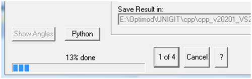
Fig. 25:
Progress display during the batch processing mode
The current
process of a batch can be cancelled by means of the "Cancel" button
if it is a sequential process. Then, the processing jumps to the next process
in the *.ubf file.
2.6.3. Further Elements
The
remaining elements are the “START” button and some information text fields above
(shown in Fig. 26). The “Show Result” is activated
when the box “Immediately” in the Settings Tab is checked (not activated =
“show off” in the example). The “Exe to run” is a placeholder for the selected
solver exe and will be updated after the “START” button is hit (here with
UNIGIT_2D). Moreover, the “Check Input” button opens the input.ctr file in
Notepad for quick control of the right setting. Finally, a text field below the
“START” button shows the elapsed computation time for the last run.

Fig. 26:
Elements around the start button
Furthermore,
the location of the diffraction angles for a given example (consisting of the
grating stack and the excitation conditions) can be output to a text file by
clicking the “Print Diffraction Angles” button.
2.7.
Show
Results Tab
This is the
last Tab in the Unigit processing order. An example is shown below (Fig.
27).
Fig. 27:
Show Results Tab
A result
file selector is located in the upper half of the tab. Files can be selected by
means of the “Add” and “Remove” buttons. The list can be completely cleared by
means of the “Remove All” button. After the list is completed, it can be
visualized in a diagram just by checking the “Show Diagram” box below (see
example in Fig. 28).

Fig. 28:
Diagram tool in the Show Results Tab
Unigit
version 2.01.02 upwards features a new diagram tool provided by UrcomTech
Berlin/ Germany. It is based on an activeX library and has to be registered
before usage.
The
implemented diagram tool offers the following options to modify the plot:
· Switching the legend on/ off by
checking/ unchecking the associated box,
· Autoscale the diagram to min/ max
range by checking/ unchecking the associated box,
· Scale the diagram by entering min/
max values for x and y (axes group),
· Change the font type and size (font
group),
· Select the active curve number # by
means of the up/down arrows (curves group),
· Change the label name of the active
curve by entering the new name into the label edit field and push the Update button,
· Change the color of the active curve
by means of the color selector,
· Change the marker type of the active
curve by means of the marker type selector,
· Change the pen size of the active
curve by means of the pen size selector,
· Delete the active curve by means of
the Delete button,
· Connect/ Disconnect curve points by
checking/ unchecking the Connect Points
box,
· Note: all changes in the curves
group have to be activated by means of the Update
button,
- Save the graph to the clip board for
further use.
In the
lower half, a check box, two buttons (Notepad and Excel) and a text field with
a selector button (“…”) to its right can be found. The text field contains the
result file (as selected in the Output Control Tab). It can be opened as text
file with the “Notepad” button. On the other hand, it is also possible to open
it directly with Excel (use the “Excel” button). In case, the German decimal
comma is activated in the system settings, the box “German CSV” should be
checked before.
3. Layer Editor
The layer
editor is closely bound to the stack editor (see section 2.4.1). The available layer types depend
on the choice of the dimension and the method. The layer editor serves for
assembling a grating stack. It is activated whenever either the button “Add” or
the button “Edit” is hit in the Grating Stack Tab. For the latter, a layer has
to be selected before. The layer editor is context sensitive depending on what
kind of grating is selected.
Unigit
offers four different basic types of stacks where each has it’s own genuine
layer types. These basic types distinguish between dimension (1D and 2D) and
method (RCWA and C-method) – see also Grating Stack Tab in section 2.4. The specific layer types of these
different gratings are discussed in the following sub-sections.They are presented
in the next sub-sections.
3.1.
Layer
Editor for 1D RCWA (1D)
Currently,
there are 9 layer types available for 1D RCWA gratings (see section 2.4.2). They fall in
five basic
and four composite types. The layer type is selected via the arrow-down button
in the drop list “Layer Type”. All layer types are presented briefly in what
follows.
3.1.1. Thin Film
A thin film
is the most elementary layer type. It consists of a flat homogeneous layer on
top of a plane underlay. Thus, it requires only two parameters for complete
description – thickness and material (see Fig. 29). In addition, an arbitrary name
can be assigned to each layer.
Fig. 29: Thin film layer
3.1.2. Rayleigh-Fourier Polygon
The editor
look for the selection of a Rayleigh-Fourier (RF) polygon is shown in Fig. 30. The Rayleigh-Fourier method is an
additional solver method beside the RCWA. It is very fast but fails if the
so-called Rayleigh hypothesis (for a sine profile with y = h*cos(kx) & k = 2pi/l holds that the method only
converges if k*h < 0.448) is violated (in many cases it works also beyond this limit).
Fig. 30:
Rayleigh-Fourier polygon
Actually,
the Rayleigh-Fourier polygon represents an interface rather than a “layer”. The
interface itself follows the polygon points in the list box. Moreover, the
materials above and below the interface (medium 1 and 2) have to be specified.
The absolute PV-value of the interface is given by the entrance in the
“Thickness” field. The z-points in the polygon list are renormalized
correspondingly. Polygon points can be added (“Insert”), removed or replaced by
means of the buttons below the list. Furthermore a polygonal interface can also
be load from a file (“Load” button). As a default, all x-values (lateral
coordinate) are normalized to 1. The absolute values are shown when the box
“abs” is checked. In addition, it is possible to check the box “trap” when the
total number of polygon points equals 6 or to check the box “blaze” when the
number of polygon points is 3. In either case, the appearance of the editor
changes from polygon point input to parametric input. The new parameters are CD
and side wall angles (SWA) for the trapezoid and only SWA for the blaze grating
(see Fig. 31).
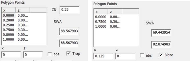
Fig. 31:
Parametric input modus for RF-polygon layer (left trapezoid,
right blaze)
In both cases, the profile can be shifted laterally by means of entering a
phase shift value for x0 (an example for the trap case is shown in Fig. 32).
Fig. 32:
Lateral shift of the RF profile by modifying x0
3.1.3. Rayleigh-Fourier Polygon
The RF Sine
is similar to the polygon (same method, similar parameters) however the
polygonal profile is replaced by a sine profile (see Fig. 33). Thus, it requires only a height (here thickness) to
specify this layer type. In addition, a lateral shift is possible by means of
the x0 input. In the example below a value of x0 = 0.1 causes a shift of 1/10
pitch to the right.

Fig. 33: RF Sine Layer
3.1.4.
RCWA
Slice, hard transition
Beside the
thin film, the RCWA slice is the most elementary layer type of the 1D RCWA
grating. One of the strengths of RCWA is that quite arbitrary and complicated
grating profiles can be put together with these slices (so-called stair case
approximation).
Fig. 34:
RCWA slice (discrete)
The
appearance of the layer editor for the RCWA slice is depicted in Fig. 34. Each slice is a slab of constant
thickness consisting of an arbitrary number of partitions (as it is called in
Unigit) meaning areas of homogeneous material that are separated by vertical
borders in the default case, i.e. skew value = 0. The partitions (and thus the
grating lines) can be skewed by entering a value different from zero (skew
angle in degrees). The location of the
border is indicated by the first column (x) in the list. The third column
contains the material descriptor. Partitions can be inserted, replaced or
deleted by means of the buttons on the bottom. In order to insert a new
partition, an x-value has to be entered and the refractive index has to be
edited.
3.1.5. RCWA Slice, soft transition
This layer
type (see Fig. 35) resembles closely the standard
RCWA-slice as described above (section 3.1.1.4). The main difference in the
appearance is that there are no discrete partitions but more or less smoothly
changing materials. This are defined in a file which has the standard extension
*f1d.
Fig. 35:
Layer editor for RCWA slice 1D, soft transition
An example
for a f1d-file is coming with the installation (unigit_grating_layer.f1d). Its
composition is rather straightforward:
- In the first line, the number
of partitions np has to be specified (must be a power of 2).
- This is followed by a
refraction index specification (i.e., 0 for direct n&k input, 1 for
reading from file, ³2 dispersion formula, see also
section 6 refraction index editor)
- Then, the information according
to the n&k specifier has to be provided, e.g., for 0 a n&k value,
for 1 a file name etc.)
- Eventually, rows 2 and 3 are
repeated np times.
Not only is
the input different compared to the hard transition RCWA slice, but there is
also a different processing. While for the standard slice with discrete
partitions consequently a discrete (analytic) Fourier transformation is
applied, a FFT is used for the soft transition. This results in a smoothing of the
material transitions across the slice. Both types enable the modelling of
volume holograms.
3.1.6.
Sliced
Polygon Layer
This layer
type is the first composite type, i.e. it is formed with standard RCWA-slices. An
example is shown below (Fig.
36). Similar to the Rayleigh-Fourier
layer types, two materials have to be specified (#1 above and #2 below the
interface borderline). The polygonal interface is described by a number of consecutive
x,z point pairs. Switching to a parametric trapezoid is likewise possible by
checking the “Trap” box. Moreover, the profile can be shifted laterally by
means of the x0 input (0.1 in the example below). As opposed to the RF-layer
types where the profile is processed as one (and thus constrained by the
Rayleigh hypothesis), the profile is sliced. The slicing itself is controlled
by the parameters “DeltaX” and “DeltaZ”. Basically, the number of slices
increases with decreasing values of those parameters. The slicing information
is stored in a sequence file and can also be reused later ().
Fig. 36: Sliced Polygon Layer
3.1.7.
Sliced
Fourier Layer
This layer
type is quite similar to the previous one. The main difference is that the profile
is specified by a Fourier formula instead of polygonal point pairs. The most
simple example is a sinusoidal interface as shown below (Fig.
37).
Fig. 37:
Sliced Fourier Layer
The Fourier formula is a definition of the
profile in terms of parametric Fourier series. Here, both the ordinate and the abscissa
are given as a Fourier series of a parameter t as follows:
Instead of
the direct input of the interface by means of point series, the coefficients ZAk
and XAk as well as the phases ZPk and XPk have
to be entered. If one would set all coefficients XAk to zero it
would lead to the known Cartesian Fourier presentation. An example for using
the first 3 even Fourier coefficients is shown in Fig. 38.
Fig. 38: Fourier composition of a profile with first 3
even coefficients
Generally,
the parametric Fourier series allows to describe rather complicated profiles
(including overhangs). An example for an overhanging is given by Fig. 39.
Fig. 39:
Overhanging profile by parametric Fourier series
For
numerical reasons, the interface description as obtained from the parametric
Fourier formula is translated into polygonal points before processing. The
number of points (input bottom center) effect both accuracy and speed.
3.1.8.
Sliced
Multi-Layer
The
previous two layer types (sliced polygon and sliced Fourier) offer a lot of
versatility specifying complicated profiles. However, they are useless when
multiple layers are interpenetrating each other. The sliced multi-layer
addresses this case. The example below (Fig.
40) shows an interpenetration of
material red, blue and white at heights between 100 and 240 nm.
Fig. 40:
Editor for sliced Multi-Layer type
The input
handling for this layer type is as follows:
- First, load a Unigit multi-layer file
(extension *.UMF),
- Second, specify the location of a sequence
file (to where the slicing information is saved),
- Then, enter a slicing criterion (#of
slices correlates with the inverse of the value),
- Following, hit “Run Slicing” to start the
slicing algorithm and
- Finally, hit “Show Slicing” to show the
sliced profile.
An example
is shown below:
'UMF File'
2
0 // '' *Direct Input*
(0.500000,5.000000) // Refraction Index
6 // # of polygon points
0.000000
0.000000
0.125000
0.000000
0.375000
0.25
0.625000
0.25
0.875000
0.00000
1.00000
0.000000
0 // '' *Direct Input*
(1.500000,0.00000) // Refraction Index
6 // # of polygon points
0.000000
0.100000
0.125000
0.100000
0.375000
0.35
0.625000
0.35
0.875000
0.10000
1.00000
0.100000
0 // 'Air' Direct Input **
(1.0,0.0) // Refraction Index
The first
line is reserved for the identifier ('UMF File'). It is followed by the
interface data in a bottom up manner, i.e., interface 1 is the bottom most one.
Each interface is described by the material below it, followed by the number of
(x,y) points and the points itself (x first, y second). It is mandatory that
the first and last y value are identical (to connect the adjacent period of the
grating). Finally, the material above the top most interface is listed.
3.1.9. Sequence
In general,
slicing information is saved into a sequence file. Thus, it serves two purposes
– first to provide the slicing for the RCWA processing of the composite layers
(see sections 3.1.1.6, 3.1.1.7 and 3.1.1.8) and second, to keep the
information for reusing in other stacks. The input mask is rather
straightforward (Fig.
41). All one has to do is to load a
sequence file (extension *.SEQ).
Fig. 41: Sequence Layer
After being
loaded, the sequence file can be either edited with a built-in tool or just
opened in a Notepad editor (where it can also be modified of course). The
built-in editor resembles closely the stack editor and is opened by clicking
the “Edit” button. Fig. 42 shows an example. The layers can be
processed in the same way as in the stack editor (see section 2.4.1) by means of the “Add Layer”,
“Edit”, “Move up”, “Move down”, “Copy”, “Cut”, “Paste” and “Delete” buttons
below.
Fig. 42:
Sequence Editor
All
thicknesses of the sequence layers are renormalized to add up to the specified
(total) thickness of the sequence layer.
3.2.
Layer
Editor for 1D C-Method (1C)
RCWA and
C-method are different modal solver methods for grating diffraction. While RCWA
is based on so-called slices by means of which almost every kind of profile can
be put together, the C-method relies on a coordinate transformation of the
profile. Therefore, the elementary “layer” types for C-method are interfaces
separated by a certain distance rather than layers having a certain thickness
as in RCWA.
Currently,
the 1D C-method in Unigit comprises 8 different layer types (see also 2.4.3). These are presented in the
following.
3.2.1.
Thin
film (plane interface)
Actually,
the term thin film is a bit misleading here for in c-method interfaces are used
rather than layers. Thus, it would be better to call this type plane interface.
An example is shown in Fig. 43. Nevertheless, a plan thin film can
by constructed by just putting two plane interfaces on top of each other.

Fig. 43:
Plane interface of 1D C-method
The input
mask is almost identical to the thin film of RCWA except there is no thickness
but a distance instead. It specifies the distance to the interface immediately
above (in case there is any).
3.2.2. CCM Polygon
The layer editor for the CCM polygonal
interface is shown in Fig. 44. There are entrances for the
corrugation of the interface (corresponding to the height of the profile) and the
distance to the next interface above. Due to the specifics of the C-method,
there are no overhanging or undercut features allowed (see /8/, /9/). The
material between the shown profile and the profile above is verified in the
refractive index entrance. Moreover, it can be chosen between absolute or
relative input of the polygonal point pairs.

Fig.
44:
Layer editor for a 1D CCM polygon layer (to be run
with C-method)
3.2.3. CCM Sinus
The layer
editor for the CCM sinus layer is shown in Fig. 45. It is very similar to the RF
sinusoidal layer, i.e., there entrances for the amplitude (thickness of the
layer) and the lateral phase X0. For the uppermost interface, the index
selection and the distance entrance are not visible. In this case, the n&k
index will be set automatically to the superstrate index that is specified in
the stack editor (see section 4).
Fig. 45:
Layer editor for CCM-sinus
3.2.4. Parallel to previous
The
parallel to previous type must not be confused with the plane interface of
section 3.1.2.1. Its input editor look is shown in Fig. 46.
It helps to
simplify the computation in case of an interface being parallel to the
interface below (which can be of any shape). Here, parallel means that the
thickness of the layer beneath (specified by the distance in the interface
below) this type of interface is constant everywhere.
Fig. 46:
Layer editor for Parallel to Previous Interface in
C-method
3.2.5. Sequence
The
sequence type is not yet available for the C-method. It is going to have a
similar meaning as for RCWA.
3.2.6. CCM Trapezoid
The
CCM-Trapezoid (see Fig. 47) is a special interface derived
from the more general CCM Polygon. It offers three parameters to define the
trapezoid profile – the CD and the two side wall angles left and right. The corresponding
polygon points are passively plotted in the polygon point list (and updated
with changing any of the parameters).
Fig. 47: CCM Trapezoid Interface
3.2.7. CCM Measurement
Likewise,
the CCM measurement interface (Fig.
48) is another special case of the CCM
polygon. However, the polygon points are read from a file rather than being
entered by means of the point list editor. To this end, a file has to be loaded
by clicking the “Load File” button on the bottom. Accepted file extensions are
*.AFM (for this type was devised to input measurement data from AFM) and *.TXT
(standard ASCII text). Examples for the file format are provided with the
installation package.
Fig. 48: CCM Measurement Interface
3.2.8. CCM Triangle
Finally,
the CCM triangle (Fig.
49) is another special case of the CCM
polygon with 3 points. Again, the profile is specified by parameters. This can
be either the two side wall angles (box “Type” is unchecked) or the base (x-coordinate
of the triangles top peak) and the corrugation (see Fig. 50).
Fig. 49:
CCM Triangle Interface – type 1
Fig. 50:
CCM Triangle Interface – type 2
3.3.
Layer
Editor for 2D RCWA (2D)
Similarly to 1D RCWA, the elementary types for this kind of
stack are layers. Currently, the 2D RCWA in Unigit offers 6 different layer
types (see also 2.4.4). These are presented in more
detail below.
3.3.1. Thin film
The thin
film layer for 2D RCWA is identical to the 1D case.
3.3.2. Patch_2D
This layer
type will be of advantage if your 2D area can be approximated by means of
rectangular patches. With the help of the editor you can specify the position
of the patch as well as its material within the elementary cell. In addition,
you need to enter the thickness of the layer. An example is shown in Fig. 51.
Fig. 51: 2D RCWA Patch layer
The
rectangles are specified by 2 diagonal corner points (x1,y1 and x2,y2) and its
material entry (by means of the refraction index editor). The embedding
material is medium 1. Note that the editor does not allow to overlap patches
(when the “Insert” button were hit in Fig. 50, the new outlined patch would not
be accepted). In general, an arbitrary number of patched can be inserted
however there is some kind of limitation from a practical point of view.
Note that unlike the super-ellipse layer, there
is no “orthogonal” option, i.e., the patch is always defined in the given
coordinate system. This means in other words that patches which have been
defined in a non-orthogonal system (pitch angle different from 0) are
parallelograms in the real world.
3.3.3. Super-Ellipse Layer
Contrary to
the patch layer type where a number of different areas can be specified, the
super ellipse layer type may include only one or two feature. However, this
feature is a less restricted one, namely a super ellipse. The mathematical
expression for a super ellipse is given below:
In case a
second ellipse is admitted, the two ellipse are allowed to overlap or to be
nested as in the example. In this case, the second ellipse overwrites the first
one. The appearance of the layer editor for an ellipse is shown in Fig. 52.
Fig. 52:
Ellipse Layer
The embedding medium is medium 1 and the
ellipse is medium 2. The dx and dy are the diameter in x and y direction
whereas sx and sy are the relative lateral shifts. Angle is the rotation angle
of the ellipse. Unlike a regular ellipse with power p = 2, the power p of a
super ellipse can be an arbitrary positive rational number. In this way, a
range of features between an ellipse and a rectangle (p = infinity) can be
covered. Moreover, a diamond can be described with p = 1 and concave shapes
with p < 1. Two cases are shown below.
In
addition, the ellipse can be rotated by specifying the wanted rotation angle
and it can be shifted laterally by entering the correspond relative values into
the edit fields sx and sy. By checking or unchecking ”Ortho” you can define
whether or not the ellipse is ”orthogonal” in real world in spite of a
non-orthogonal cell (defined by zeta – see stack editor). For further
explanation see also the drawing below.
Check the
box Ortho if you want to have an ellipse in real world, otherwise the ellipse
is defined for the non-orthogonal coordinate system, i.e., it will be distorted
in real world. Schematically, this is shown in the drawing below (Fig.
53). Notice, the drawing in the editor
(see Fig. 52) does not show this, however, your
calculation result is supposed to be different for the cases of a checked and
an unchecked Ortho box.

Fig. 53:
Orthogonal and Non-Orthogonal shape of the ellipse
in a non-orthogonal coordinate system.
3.3.4. Fill 2D Layer
Unigit offers a feature for arbitrary pixel filling of
a 2D layer. It is comparable to the gradient RCWA (or soft slice) in 1D. If you
want to include an arbitrary fill layer then pick the Fill2D option in the drop down box of the 2D layer editor.
Then, the layer editor opens with the window shown in Fig. 54.
Fig. 54:
Fill 2D Layer Editor
Here, you need to specify the layer thickness and you
can enter a name for the layer similar to other layer types. Moreover, you need
to specify a material for the embedding medium and a file (with the extension
*.f2d) which contains the bitmap description of the layer.
The file content is explained as follows:
2 /number
of materials beside the embedding material
0 /specification
ID for material 1 (0 = direct input)
1.5 0.0 /n&k
for material 1
1 /specification
ID for material 2 (1 = n&k file)
'C:\Program Files\OPTIMOD\Unigit\NKData\SILICON.NK'
/pathname of the n&k file for material 2
6 97 /Fourier
discretization power (e.g., discretization is 2^6) & number of lines to
follow
528 0 /pixel
number & material ID, e.g., 528 pixels with material 0 (embedding material)
32 1 /pixel
number & material ID, e.g., 32 pixels with material 1
32 2 /pixel
number & material ID, e.g., 32 pixels with material 2
……..
32 1 /pixel
number & material ID, e.g., 32 pixels with material 1
528 0 /pixel
number & material ID, e.g., 528 pixels with material 0 (embedding material)
Note, the total number of pixel description lines in
this example must be 97 and the total number of added pixel numbers (i.e., 528
+ 32 + 32 + … + 32 + 528) must be equal to (26)2 = 4096.
A graphical example for a non-orthogonal cell is shown
below. First, the elementary cell has to be defined as shown (red
color in Fig. 55).
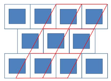
Fig. 55:
Determination of the elementary cell
As a next step, one has to do the
discretization in unit cell coordinates. The linear pixel number has to be a
power of 2 (64, 128, 256 etc.). The pixel number in both axes has to be the
same (no matter what the pitch is).

Fig. 56:
Filling of an arbitrary layer
The counting direction is indicated by the
green arrows in Fig. 56, i.e., scanning row by row with
blanking like behaviour (jump from the end of one row to the begin of the next
row) as shown. As long as pixels have the same material (defined by largest
area percentage) just add, when material is changing ® save the value and restart counting
(across scan blanking).
This would result in the following *.f2d
information for the graphical example assuming material 0 is white and material
1 is blue:
48 0 (3
lines with 16 pixel each)
3 1 (3
pixels blue)
6 0 (6 pixels white)
10 1 (7 pixels in row #4 right hand and 3 pixels
in row #5 left hand, counting across the blanking)
5 0 (5 pixels white)
etc.
The
installation of version 2.02.02 comes with 3 stack files that describe all the
same geometry (a rectangular area with n = 1.5 embedded in vacuum with n = 1)
but with different means:
·
stack2d_elli.ust using the ellipse descriptor (ellipse
filling),
·
stack2d_arbi.ust using the new bitmap descriptor
(arbitrary filling),
·
stack2d_rect.ust using the patch descriptor (patch or rectangle
filling).
Running
these files should give very similar results (for details see Unigit tutorial).
3.3.5. Cone 3D
This layer
type permits to insert real 3D structures by means of a very compact
description. It is quite similar to the 1D composite layer types in the sense
that an automatic slicing works behind the scenes to transform the input
description in a number of 2D slices of the 2D ellipse layer type. It is
activated by selecting the CONE-3D option in the 2D layer editor. In doing so,
the layer editor window as depicted in Fig. 57 shows up.

Fig. 57:
3D Cone Layer
Here, the user can define the top and the
bottom cross section shape of his grating pattern just like the same way as he
is used to with the ellipse filling feature. But as opposed to it, now a real
3D body is defined. The vertical shape of this body is defined by the vertical
power. Here, a 1 results in a straight line while a value >1 gives a convex
and a value <1 results in a concave shape, respectively. Furthermore, the
user can define the number of slices. Actually, an equidistant slicing routine
takes care to automatically translate the compact 3D description in something
digestible for the RCWA solver. Finally, the user can sweep up and down through
the 3D body by means of the “Show Slice” option. Here, the cross section shape
of the activated slice number is plotted. Fig. 58 shows such a sequence of cross
sections for the body defined above.
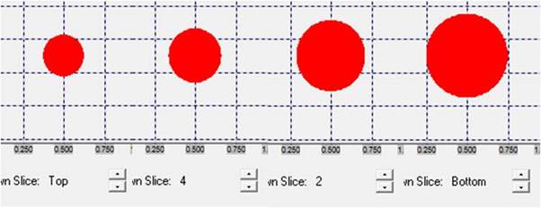
Fig.
58:
Sequence of cross sections when vertically sweeping
through a 2D composite layer
3.3.6. Sequence 2D
The layer type sequence just like the type thin
film layer is common for 1D and 2D. The difference is that a 1D sequence can
only contain 1D layer types whereas a 2D sequence has to contain 2D layer types
only. However, the appearance of the layer editor will be the same. Basically,
a sequence can only be used if defined before. If a sequence layer is to be
built into a stack, the location of the stored file has to be specified in the
corresponding edit field. In addition, the total thickness of the sequence has
to be entered. The structure of the sequence (or sub-stack) is renormalized to
this thickness. Likewise, the lateral dimensions are renormalized to the new
pitch (grating period). The button EDIT
permits to edit the sequence in the stack editor whereas the button Notepad
opens a notepad with the sequence in ASCII-format.
3.4.
Layer
Editor for 2D C-Method (2C)
Similarly to 1D RCWA, the elementary types for this kind of
stack are layers. Currently, the 2D RCWA in Unigit offers 6 different layer
types (see also 2.4.4).
Presently,
there are four interface types implemented with the restriction that only a
stack with parallel interfaces can be processed. This means that except of the
bottom interface (that has to be of type pyramide, micro-lens or fill 2C) all
interfaces above have to be of type parallel layer (see section 3.4.1).
All
interface types are presented in more detail below.
3.4.1.
Parallel
Layer
The parallel
interface for 2D C-method (Fig.
59) is identical to the 1D case.
Parameters to input are the material (above the
interface) and the distance to the interface above (if there is any).
Fig. 59:
Parallel Interface for C-method 2D
3.4.2. Pyramide Layer
The pyramide
interface (Fig. 60) is characterized by its Top CD in
x & y (TCDx, TCDy), its bottom CD’s (BCDx, BCDy), its height and the
rotation angle (describing the tilt of the pyramide relative to the elementary
cell of the grating. Additional parameters to input are the resolution
(required for the FFT during processing), the material above and the distance
to the interface above. Moreover, the checkbox “Inverse” offers to turn around
(i.e. to put it upside down) the pyramide. A false color plot in the lower
right half shows the shape synchronously.

Fig. 60: Pyramide interface
3.4.3. Micro-lens Layer
This
interface allows the modelling of a micro-lens array. The required parameters (see
Fig. 61) are the lens radii in x and y
direction (Rad x & Rad y), the conical constants (Con x & Con y) and
the height of the micro-lens. Again, a resolution for the FFT and a rotation
angle (defining the relative tilt of the lens w.r.t. the elementary cell) can
be entered. Also, the micro-lens can be inverted, i.e. showing upside down. The
footprint of the lens is calculated and displayed in the Edge x & y fields.
Like for all other 2C layers, the material above the interface and the distance
to the interface above have to be specified.
Fig. 61: Micro-Lens interface
3.4.4. Fill 2C Layer
This
interface type is devised to enable the input of an arbitrary 3D surface into
the 2D C-method algorithm. This is achieved by loading a surface fill file
(extension *.F2C). After the file is loaded, the surface is shown in a false
color plot (red = high and blue = low heights) on the lower right. Moreover,
the height, the distance to the interface above and the refraction index have
to be entered into the editor mask (Fig.
62).
Fig. 62:
Fill 2C Interface
The
structure of the *.F2C surface file is as follows:
- First line: FFT number
- Next FFT*FFT lines: height values
The height
values are relative. They are normalized with the height value to be input into
the “Height” edit field.
4. Refractive Index Editor
The n&k editor serves the definition of the
refraction indices of all materials needed to build the layer stack, i.e., the
substrate, the superstrate and all kinds of layers between. It is available
wherever required within the stack editor. To call the editor one has simply to
click the related EDIT-button.
Related to the three basic possibilities of
describing the materials, the appearance of the editor changes correspondingly.
After being called, it comes always up in the direct refraction index input
mode. Other selections can be straightforwardly made by choosing the wanted
option in the drop down box. This is shown in Fig. 63 along with all the possible
options.

Fig. 63: Selection of the refraction
index input mode
The
available selections fall into three basic options:
- Beside the direct input, one
can
- get the refractive index from a
file,
- or have it computed from a
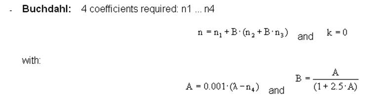
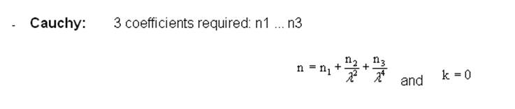
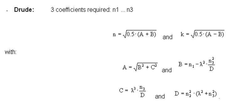
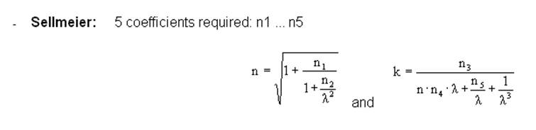
certain dispersion formula (Buchdahl, Cauchy etc.).
4.1.
Direct
n&k Input
The direct refraction index input mode is shown
in Fig. 64.
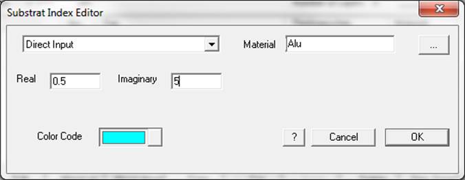
Fig. 64: Refraction index editor
Here, the real and the imaginary part of the refraction
can be inserted directly. Then, these values are assumed to be constant for all
related calculations no matter what wavelength was specified. Apparently, in
this way no dispersion is taken into account.
Moreover, a material ID can be assigned. While
entering an ID name, Unigit checks the color table (see section 3.2) for this name and if being found
presents the color assigned to it.
4.2.
File
Input
If you pick the file input, the index editor will have
the look depicted in Fig. 65.
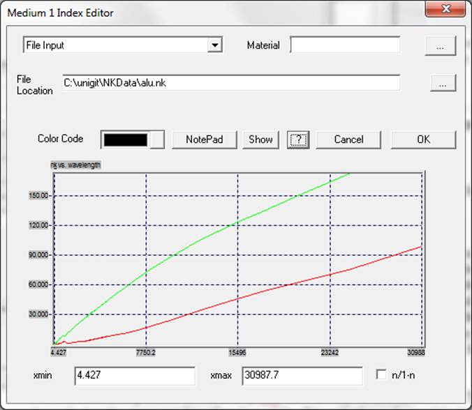
Fig. 65:
Refraction input via nk-file selection
Here, the complete path name of the file with
the required index data has to be specified. This can either be done by typing
the pathname into the corresponding field (file location) or by clicking the
file request button (marked by “…”). In the letter case a file selection box
pops up and one has to make a choice. Of course, the file location is not
fixed. However, it is recommended to use the folder
"...\Unigit\NKData" that is generated during the installation of the
UNIGIT code. Basically, the file extension "*.nk" is preferred. The
Unigit installation comes with a couple of *.nk example files. Feel free to
complete this library according to your needs.
After having specified the n&k file, the
data are loaded and shown in a diagram (n red & k green). Alternatively,
the n/(1-n) presentation can be chosen for EUV or x-ray materials by checking
the corresponding box. Concurrently, the wavelength range as read from the file
is given (xmin & xmax). It is possible now to zoom in by changing these
values.
Furthermore, it is possible to connect a
n&k file directly with a material ID. This can be done by replacing the comment
line (first line of the file) with the code word "color" followed by
a colon and the material ID name (see example below in Fig. 66). Then, when the n&k file will
be used somewhere in the stack, Unigit checks the comment line, when
identifying a material ID compares it with the colour table and when successful
assigns a colour to it.
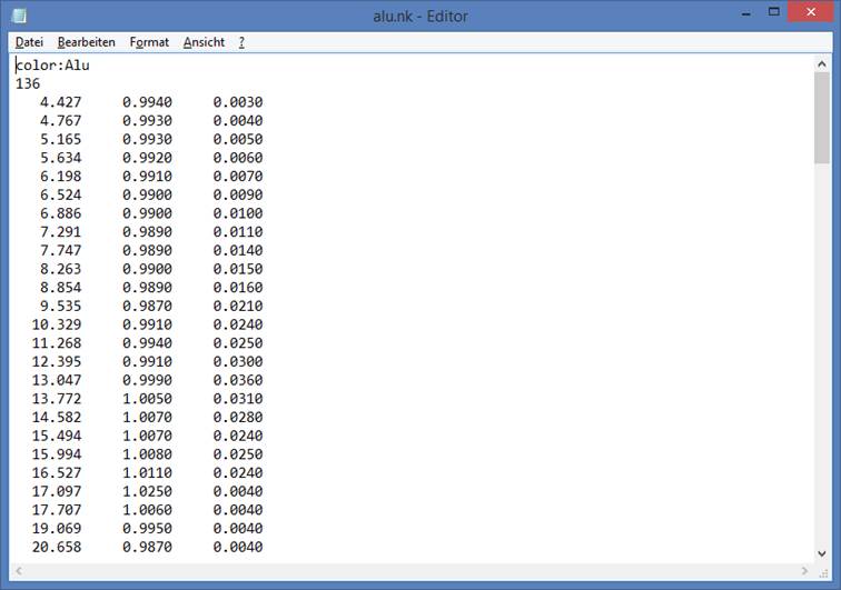
Fig.
66: n&k
file listing with material ID for color coding (indicated by key word "color:")
4.3.
Dispersion
Formulas
Eventually,
the refractive index can be defined by means of a certain dispersion formula.
Then, the input mask looks like shown in Fig. 67.
Fig. 67:
Refraction input via dispersion formula
Depending on the selected dispersion formula,
the coefficients n1 thru n3, n4 or n5 as required by the related dispersion
formula have to be entered. Make sure that the coefficients are related to the
wavelength as given in microns rather than nano-meter, Angstrom or other length
measures. Another possibility is to select a certain coefficient set from the
combination field. In addition, once the coefficients are entered, the present
coefficient set can be saved. In order to be able to recall the set properly, a
name has to be entered in the select box. Then, it is available under this name
for future operations. If it is not needed anymore, it should be deleted again.
The coefficient information is stored in one file per dispersion formula (with
the related file name). These files are also located in the folder
"...\Unigit\NKData" and can be identified by the file extension
".nkk".
A list of
the available dispersion formulas is shown below:


5.
UNIGIT Projects
5.1. General Remarks
Unigit project files have been introduced to
facilitate the organization of complex modeling projects as well as to give some
support in retrieving and reconstructing simulations dated back some time.
Concurrently, it provides an appropriate mean to avoid time consuming reruns of
the UNIGIT solver in order to obtain the results in a different output format
for the same application example. Suppose for instance, you have calculated the
diffraction efficiencies for a complex 2D example that took several hours.
Later, it turns out that you also need the phase information. Then, it would
have been a good idea to activate the project file generation in the first run
(see section 2.5.5).
In the
grating stack tab (section 2.4), Unigit project files can be
loaded instead of stack files (see Fig. 68). They possess the extension “*.UPR”.

Fig. 68:
Selection of an Unigit project file
After
selecting an UPR file, UNIGIT switches from its regular mode into the project
retrieval mode. This becomes obvious by two features:
First, the group in the upper right corner
changes its name from “Stack” to “Project” and secondly, the START button
changes its name into “Extract Results”. In addition, the buttons in the project
control group (middle right) are enabled (see Fig. 69).
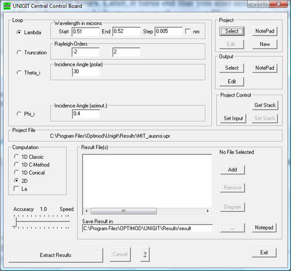
Fig. 69:
Appearance of the central control board in project
retrieval mode
5.2.
Retrieving input information
The input
information is simply retrieved by clicking the button SET
INPUT in the group “Project Control”. Then,
all input masks such as “Lambda”, “Truncation”, “Theta_i” and “Phi_i” are
updated with the original state used to generate the active project file.
Likewise, the loop setting is updated along with the associated start, stop and
step parameters.
5.3.
Retrieving
stack (grating) information
The retrieval of the original stack information
is a two-step procedure. In the first step, the stack information is retrieved
and saved to a file by means of the GET STACK button. To this end, a file name has to
specified by means of the output editor (see section 7.3). After successful operation, the SET STACK button is enabled.
In the second step, the stack file can be set
as active stack file and the basic operation mode of Unigit can be switched
back to regular by clicking the SET STACK
button. Concurrently, Unigit identifies whether the stack file is a valid
Unigit format and issues an error message if this is not the case.
5.4.
Retrieving
computation results
Another very important functionality of
UNIGIT’s project retrieval mode is the generation of arbitrary result
information from a given project file. This is simply done by clicking the EXTRACT RESULTS button. The way how the output is
organised has to be set in exactly the same way as for the regular mode. Again,
this is done by means of the output editor (see section 7.1) in exactly the same way as for the
regular mode. Actually, one will see only subtle change in appearance when
starting the output editor (described elsewhere). In addition, some options
will be disabled (output only in one file). Analogously, either single files
(one for each diffraction order), one big file (all in one) or no file meaning
the output is displayed in a DOS window can be generated. The essential
difference is that the information is retrieved from a sort of archive (UPR
file) instead of being generated by a solver. Thus, it is much faster. Of
course, all on board features for data exploration, i.e., starting a notepad to
display the ASCII formatted result files or the diagram feature can be applied
the usual way (see section 2.5).
6. Miscellaneous
6.1. Command Line Operations
6.1.1.
General
Remarks
All Unigit
computation kernels can be run from command line skipping the GUI. In order to
do so, run a cmd window, change to unigit installation folder and call the
unigit exe you want to run along with 3 or 5 parameters. The parameters are:
- parameter 1: either wavelength (in
microns), AOI, azimuth or truncation (depends on parameter 2) - overwrites
the entrance in input.txt (see section 9.2),
- parameter 2: defines interpretation of
parameter 1: 0 - wavelength, 1 - truncation order, 2 - AOI, 3 – Azimuth,
- parameter 3: number of the thread for
parallel mode (1 through n) or 0 in sequential mode,
- parameter 4 (optional): same selection as
for parameter 1, i.e., a second "loop" parameter can be selected
in this way,
- parameter 5 (optional): defines the
interpretation of parameter 4 (meaning see parameter 2)[1].
The
parameter passing is required for the GUI for looping and parallelization. All
unigit kernels are controlled by the information in unigit.ctr (it is hard
coded). It has to be in the same folder as the exe. The unigit.ctr file is a
sort of pointer to the files that control the unigit run. It contains only
three lines with the following meaning:
- line 1: input control (see section 9.2)
- line 2: stack file - it is urgently
recommended to generate the stack file with the unigit stack editor (see 4). Only very experienced users
are encouraged to generate it by other means.
- line 3: the output control file (see
section 9.3).
6.1.2. Input Control
The lines
of the input control file have the following meaning:
- line 1: minimum truncation order
- line 2: max truncation order
- line 3: AOI in degrees
- line 4: azimuth in degrees
- line 5: wavelength in microns
- line 6: TE computation required (bool) -
applies only to unigit_1d, unigit_1C
- line 7: TM computation required (bool) -
applies only to unigit_1d, unigit_1C
- line 8: speed/ truncation shape identifier
(0 is standard RCWA with rectangular truncation - best accuracy, least
speed vs. max 2.5 least accuracy, highest speed) applies only to unigit_2d
and unigit_2dsx
6.1.3. Output Control
The lines
of the output control file have the following meaning:
- 1. line:
lfout (bool): file output if .t., no file output if it is .f.
- 2. line: iout (int): 0=r&t (one file),
1=r,2=t,3=r&t,4=r(one file),5=t(one file), >0 -> append, <0
-> new
- 3. line: l_info(bool): show additional
information how the algorithm is processed
- 4. line: path of the result file(s) (if
any)
- 5. line i_eff (int): defines the type
of output: 0=efficiency, 1=eff
& phase, 2=amp & phase, 3=phase, 4=joint eff(coni), 5=elli,
6=cmplx, 7=angles
- 6. line: lpercent (bool) output in percent
(.t.) or output in relative to 1(.f.)
- 7. line: nop_min x (int): minimum order to
output (applies for 1D and 2D)
- 8. line: nop_max x (int): maximum order to
output (applies for 1D and 2D)
- 9. line: nop_min y (int): minimum order to
output in y direction (applies only for 2D)
- 10. line: nop_max y (int): minimum order
to output in y direction (applies only for 2D)
- 11. line: fname_rte: if different from '0'
- the complete diffraction matrix for TE-polarization reflection is
written out to the a file or location with the entered name (applies only
to unigit_1D)
- 12. line: fname_rtm: if different from '0'
- the complete diffraction matrix for TM-polarization reflection is
written out to the a file or location with the entered name (applies only
to unigit_1D)
- 13. line: fname_tte: if different from '0'
- the complete diffraction matrix for TE-polarization transmission is
written out to the a file or location with the entered name (applies only
to unigit_1D)
- 14. line: fname_ttm: if different from '0'
- the complete diffraction matrix for TM-polarization transmission is
written out to the a file or location with the entered name (applies only
to unigit_1D)
- 15. line: Output Format (int) : 1 = float,
8 digits; 2 = float, 4 digits; 3 = fix, 8 dig; 4 = fix, 4 dig; 5 = science,
8 dig; 6 = science, 4 dig
- 16. line: generate project file (bool): if
.t. - an unigit project file is output (about .upr files and handling see
section 8)
- 17. line: path of the unigit project file
(.upr)
6.2.
Calculation
of the Diffraction Angles
Basically,
Unigit offers two different options for the calculation of the diffraction
angles. The first quick option can be done upfront and does not need to run the
RCWA- or C-method computation kernels. It can be launched by clicking the
button SHOW ANGLES. The results are shown
immediately in a Notepad window. An example is inserted in Fig. 9 for a dielectric grating (nsubstrate
= 1.5) with pitch = 1 micron at l = 0.5 and AOI = 45°.

Fig. 70:
Presentation of diffraction angles
In the second option, the angular information
is a by-product of a full computation run. In order to access it, one has to check
the “Diffraction Angles” box in the Output Control Tab (see section 2.5.4).
The angles are defined according to Fig. 71. The polar angles q are measured between the normal axis z and the
incident or diffracted ray. The azimuthal angles j are measured between the projection
of the ray into the x-y plane and the x-axis.
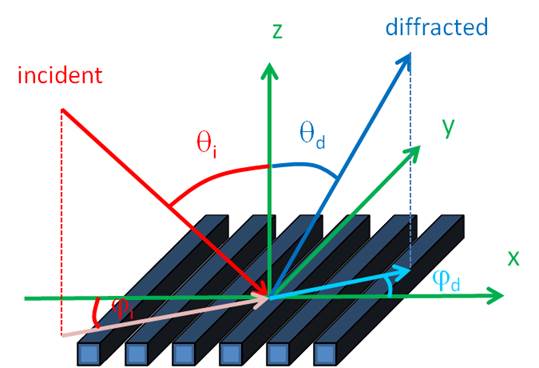
Fig.
71:
Definition of the incidence and diffraction angles
in Unigit
References
/1/ M.G. Moharam, D.A. Pommet and E.B. Grann:
“Stable implementation of the rigorous coupled wave analysis for surface-relief
gratings: enhanced transmittance matrix approach”, J. Opt. Soc. Am. A 12
(1995), pp. 1077-1086.
/2/ Lifeng Li, “Multilayer modal method for
diffraction gratings of arbitrary profile, depth, and permittivity,” J. Opt.
Soc. Am. A 10 (1993), pp. 2581-2591.
/3/ D. Agassi and T.F. George, “Convergent schema
for light scattering from an arbitrary deep metallic grating,” Phys. Rev. B 33 (1986), pp. 2393-2400.
/4/ Lifeng Li, “Formulation and comparison of two
recursive matrix algorithms for modeling layered diffraction gratings,” J. Opt.
Soc. Am. A 13 (1996), pp. 1024-1035.
/5/ Lifeng Li, “Use of Fourier series in the
analysis of discontinuous periodic structures,” J. Opt. Soc. Am. A 13 (1996), pp. 1870-1876.
/6/ Lifeng Li, “New formulation of the Fourier
Modal Method for crossed surface-relief gratings,” J. Opt. Soc. Am. A 14 (1997), pp. 2758-2767.
/7/ P. Lalanne, “Improved formulation of the
coupled wave method for two-dimensional gratings,” J. Opt. Soc. Am. A 14 (1997), pp. 1592-1598.
/8/
J. Chandezon, D. Maystre and G. Raoult, “A new theoretical method for
diffraction ratings and its numerical application,’’ J. Opt. (Paris) 11,
235–241 (1980).
/9/
L. Li, J.
Chandezon, G. Granet, and J.-P. Plumey, “Rigorous and efficient grating analysis method
made easy for optical engineers,” Appl. Opt. 38, 304-313 (1999).
/10/ J. Bischoff, “Improved
diffraction computation with a hybrid C-RCWA method,” Proc. SPIE 7272, part 2
(2009).
See e.g. http://www.osires.biz/page6.php - reference #5
Acronyms
AOI - Angle of Incidence
AR - Anti Reflective
BARC - Bottom
Anti Reflective Coating
CCB - Central Control Board
CD - Critical Dimension
CM - Coordinate Transformation Method (a.k.a. C-method)
GUI - Graphical User Interface
PR - Photo resist
RCWA - Rigorous
Coupled Wave Approach
RF - Rayleigh-Fourier (Method)
TE - Transverse Electric
TM - Transverse Magnetic
1D - one-dimensional
2D - two-dimensional
3D - three-dimensional
The project
retrieval mode is activated when loading a project file instead of a stack
file. In the output editor, this becomes visible by the name change from
“Project File” (compare section 7.1) to “Stack File” (see figure
below).
![]()

In case you want to retrieve the stack file from a Unigit project file (see
section 8.3), you have to check this box and
enter a file name where to save the stack information to. The default extension
is the standard “.ust” if not specified otherwise.